Building-block flows: a modular approach to turbulence modeling
A new machine-learning model learns the physics of turbulence from simple canonical flows and uses it to predict the aerodynamics of real aircraft.
Designing the next generation of fuel-efficient aircraft, trucks, and ships requires thousands of virtual experiments. Engineers use computational fluid dynamics (CFD) to test new shapes and configurations before building physical prototypes. In principle, this could save years of development and billions of dollars in wind tunnel campaigns.
The problem is that these simulations are only as good as their underlying models. Turbulence, the chaotic swirling motion that dominates most real-world flows, spans an enormous range of scales. Resolving all of them in a simulation would require computational grids with trillions of points — far beyond what any computer can handle today. So we rely on models that approximate the effects of the scales we can't afford to resolve. And these models, despite decades of development, still fall short of the accuracy demanded by industry.
In our paper published in Communications Engineering, we introduce the Building-block Flow Model (BFM), a closure model for wall-modeled large-eddy simulation (WMLES) that takes a fundamentally different approach to this problem.
The core idea: complex flows are built from simple ones
Think about how a child learns to read. They don't start with novels: they learn the alphabet first, then words, then sentences. Once they master the building blocks, they can read texts they've never seen before.
The BFM follows a similar philosophy. Instead of training on complex geometries like wings or aircraft, the model learns the physics of turbulence from a handful of building-block flows: simple flows that capture fundamental physical regimes. These include flows under zero, adverse, and favorable pressure gradients, as well as separated flows. The hypothesis is that these canonical configurations encapsulate the essential small-scale physics that a closure model needs, and that this knowledge generalizes to far more complex scenarios.
This deliberate simplicity is a feature, not a limitation. By avoiding training on geometries resembling the test cases (no airfoils, no bumps, no wings), we prevent the model from merely memorizing specific configurations. Instead, it must learn the underlying physics—and that physics turns out to be transferable.
One model
Traditionally, WMLES requires two separate models: a wall model that provides boundary conditions at solid surfaces, and a subgrid-scale (SGS) model that accounts for unresolved turbulence in the interior of the flow. These models are typically developed independently, which can lead to inconsistencies.
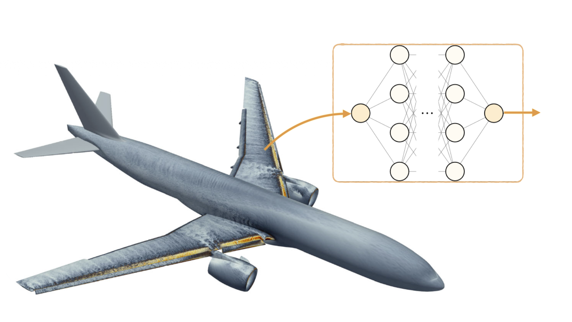
The BFM unifies both into a single framework implemented through three feedforward artificial neural networks (ANNs). The first ANN predicts the wall-shear stress at solid boundaries. The second handles the SGS stress in the cells immediately adjacent to walls, where the interaction between the wall model and the SGS model is most critical. The third ANN models the SGS stress everywhere else. The inputs to all three networks are the local invariants of the velocity gradient tensor — quantities that are independent of the coordinate system and therefore applicable to any geometry.
Training data that respects the numerics
One of the most subtle challenges in developing data-driven turbulence models is the mismatch between the "ideal" training data and the reality of a numerical simulation. Most ML-based SGS models are trained on filtered direct numerical simulation (DNS) data. But in practical WMLES, the grid is so coarse (often 100 to 10,000 times larger than the smallest flow scales) that numerical errors become comparable to the modeling errors themselves. A model trained on perfect data may perform poorly in an imperfect numerical environment.
To address this, we generate training data using a technique called exact-for-the-mean WMLES. The idea is to run WMLES of the building-block flows in the same solver and on the same type of grid that will be used in production simulations, but with an eddy viscosity that is iteratively adjusted so that the simulation reproduces the correct mean velocity profiles and wall-shear stress from high-fidelity DNS data. The resulting training data inherently accounts for the numerical discretization, ensuring consistency between the model and the solver.
From pipes to aircraft
We validated the BFM across five progressively complex cases, comparing its performance against established models:
Turbulent pipe flow. Here the Reynolds number is far beyond the training range. The BFM predicts the wall-shear stress within 3% of experimental measurements, while classical models overshoot by 22%.
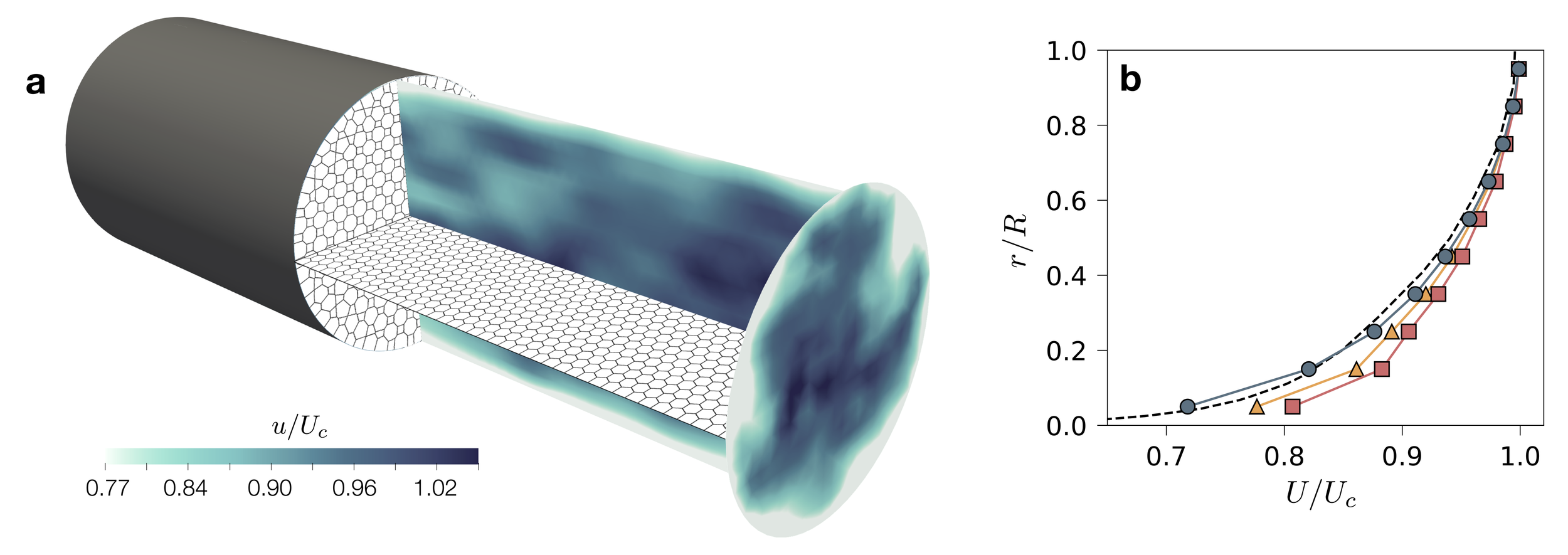
Numerical simulation of a turbulent pipe flow in a coarse grid. (a) Grid and instantaneous velocity in the pipe. (b) Mean velocity profile: high fidelity simulation (dashed line); BFM (blue circles); and classical models: Vreman model (yellow triangles), and Dynamics Smagorinksy model (square).
Separated flow over a Gaussian bump. This Boeing-designed test case has been notoriously challenging for both RANS and LES. On a grid with roughly 9 million cells, the BFM correctly predicts the flow separation and the counter-rotating vortex structure downstream of the bump. Classical models fail to predict separation entirely, overestimating mean velocities by more than 30%.
NASA Juncture Flow. This simplified aircraft features flow separation at the wing-body junction. BFM yields improved mean velocity predictions at all measurement locations compared to classical models.
NASA CRM-HL (aircraft in landing configuration). This is the gold standard benchmark for the aerospace community — a geometrically realistic aircraft with deployed flaps, slats, and a flow-through nacelle. The BFM provides similar or better accuracy in lift, drag, and pitching moment coefficients, particularly at high angles of attack near stall. Crucially, the BFM achieves this despite having never seen an aircraft-like flow during training.
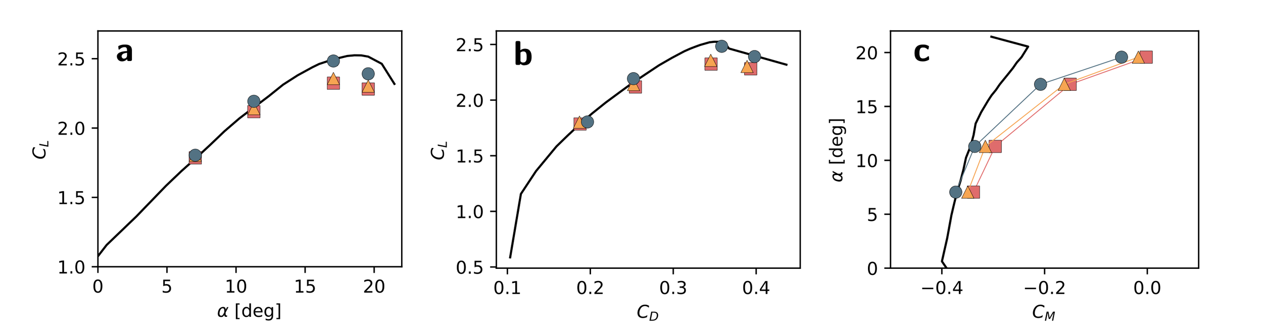
Results for the NASA CRM-HL. (a) Lift coefficient (CL) as a function of the angle of attack of the aircraft (b) Drag coefficient (CD) vs lift coefficient. Pitch moment coefficient as a function of the angle of attach. Results from experiments (black line); BFM (blue circles); and classical models: Vreman model (yellow triangles), and Dynamics Smagorinksy model (square).
What about computational cost?
A practical model must not only be accurate but also affordable. The computational cost of running WMLES with BFM is approximately 0.9 times that of DSM-EQ and 1.1 times that of VRE-EQ — essentially the same. The model is implemented in CUDA for GPU architectures, leveraging the fact that neural network evaluations are naturally parallelizable on GPUs.
For the Gaussian bump, the BFM achieves comparable accuracy to DSM-EQ on a grid with 52 times fewer control volumes (9 million versus 452 million), representing a massive reduction in computational resources.
Looking ahead
Perhaps the most exciting aspect of the BFM is its modularity. The current version accounts for zero, adverse, and favorable pressure gradients, as well as separation. But the framework is designed to grow: future versions can incorporate additional building blocks for compressibility, shock waves, wall roughness, laminar-to-turbulent transition, and more. This scalability is absent in traditional SGS models, whose functional forms are fixed at the time of their design.
Truly revolutionary improvements in WMLES will require simultaneous advances in numerics, grid generation, and modeling. The BFM addresses all three by devising models that are consistent with the numerical discretization and the grid structure of the solver. We believe this integrated approach, combined with the scalable building-block philosophy, opens up new opportunities for developing closure models that are both accurate and broadly applicable.